Adaptive Thresholding for Document Image Binarization
Binarization is the process of converting a colour or grayscale image into a binary (i.e. black and white) image. It’s typically the first step performed by software that does any sort of document analysis and recognition, optical character recognition (OCR) being the most common application. When a document is scanned with a flatbed scanner, well established algorithms do a very good job. Nowadays, however, many document images come from the cameras in our mobile devices, and these are subject to variable lighting conditions that make binarization quite difficult. The problem is exacerbated when capturing images of bounded pages because the binding often prevents pages from laying flat, thus accentuating lighting variation.
One of my pet projects is Music Lens, which is similar to OCR but for sheet music rather than text. Music Lens runs on iOS, so it’s designed to work with images obtained from the device’s camera. The quality of the binarized image has a huge impact on the overall accuracy of Music Lens, so I’ve invested a lot of time trying to find the best binarization algorithm. To this end, I’ve been reading academic research papers, implementing some of the best algorithms, and experimenting with some variations. The final algorithm I’m now using isn’t entirely new, but combines several techniques described in the literature in a new way. (Or, at least I think so. I haven’t done an exhaustive reading of the literature, so the algorithm might already be published elsewhere. If any reader finds a research paper that describes the same technique, please let me know.)
There are three main parts to this article:
-
First, a brief review and example of Otsu’s method [1] is given. This is probably the most common “established” binarization method. No effort to explain Otsu’s method is given, as innumerable sources already do this. To provide justification for the following sections, an example where Otsu’s method fails is provided.
-
In the second part, I describe a more advanced algorithm from the research literature that I selected and implemented for Music Lens. This algorithm worked exceptionally well in my initial experiments, but then later I discovered short-comings that became evident when I changed how I was taking pictures with my iPhone.
-
In the final part I explain a new algorithm that uses several ideas I gleaned from the research literature.
Notation
I’ll use \(I: \mathbb{N}^2 \rightarrow [0, 255]\) to represent the original grayscale image and \(J: \mathbb{N}^2 \rightarrow \{0, 1\}\) to represent the computed binary image obtain from \(I\). \(I(x, y)\) refers to the pixel value of the image \(I\) at the coordinate \((x, y)\).
Background
Binarization algorithms are generally categorized as either global or adaptive. A global technique applies a single threshold value \(t\) to compute the binary image as
The essence of a global thresholding algorithm is in how \(t\) is determined.
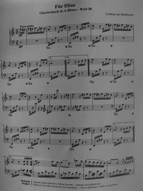
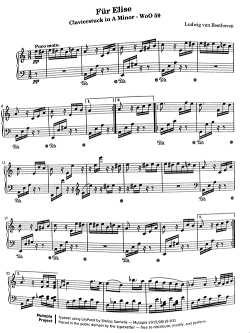
The most famous global thresholding technique is known as Otsu’s method. Otsu’s method assumes that the image \(I\) is dominated by pixels that cluster around two values, which represent the foreground and background colours. When this condition is met, the histogram of pixel levels is bimodal (i.e. has two distinct humps). Consider the image in Figure 1:
Image of one page of a music score captured in a well-lit environment.
Here is the histogram of the graylevels:

The graylevel histogram for the image in Figure 1.
The smaller hump on the left corresponds to the black-ish foreground pixels and the larger hump on the right corresponds to the white-ish background pixels.
The large hump on the right corresponds to the background pixels, and the smaller hump to the right corresponds to the foreground (blackish) pixels. Conceptually, Otsu’s method selects a threshold value \(t\) that best separates the foreground and background pixels. By visual inspection of the histogram, it’s clear that \(t\) should be somewhere between the peaks of the two humps—that is, somewhere between 40 and 210. According to Otsu’s method, the optimal value of \(t\) is 132. When we apply Otsu’s method to our score above (Figure 1), we get this:
The result of applying Otsu’s method.
This result is pretty good, but it also reveals a key weakness with all global methods: when the foreground or background varies, there is no choice of \(t\) that yields satisfactory results. Here we see that in the original image (Figure 1) the lower-right corner of the page is a bit darker than everywhere else, and in the binary image (Figure 3) we end up with a blotch of black. In this particular case we were lucky and the resulting image is still usable because the blotch is away from the actual music notation. But, as shown below, global methods like Otsu’s can fail catastrophically on images with more variation, as illustrated in Figure 4:
An example of when Otsu’s method (or any global thresholding method) will fail catastrophically.
Because the left side of the page is much darker than the right side, there’s no single value for \(t\) that can binarize this image correctly.
A better algorithm is needed.
Current Methods
Document binarization is an active area of research and since 2009 the academic community has held annual competitions to evaluate and highlight the state-of-the-art in the field. These competitions are known as DIBCO (for Document Image Binarization Contest). There doesn’t appear to be a single website for DIBCO, but if you google “dibco binarization” you’ll find information about DIBCO for recent years. Current research efforts are focused on binarizing badly illuminated documents, handwritten documents, and historical documents. All the test images used in the competitions fail horribly with global methods like Otsu’s.
Otsu’s method remains an important technique, however. In the 2009 DIBCO competition, at least 13 of the 43 submitted algorithms use Otsu’s method in some form. One common approach employed is to estimate the background and then applying Otsu’s method on a normalized image.
One such method is from Singapore researchers Lu and Tan and described in their paper Thresholding of Badly Illuminated Document Images through Photometric Correction [2]. (As far as I know, this algorithm was never submitted to any DIBCO competition. It’s worth noting though that the authors did win the 2009 DIBCO with an improved algorithm also based on background estimation.) Their algorithm is fast and intuitive. First, the background is estimated by fitting a bivariate polynomial of degree 3 (or higher). This polynomial is then used to normalize the image, removing the variation in the background intensity. Otsu’s method is then applied to the normalized image.
Let’s apply this method to the first image from Figure 3 that failed with Otsu’s method. The first step is to estimate the background with a polynomial. Conceptually, we want to think of the image existing in 3D space, with the pixel values providing the \(z\) coordinate (the height). We estimate the background polynomial by using least squares fitting on a set of sampled points \(\{(x, y, I(x, y))\}\). When we do this for the image above, we get this polynomial:
This is what \(B\) looks like:

A 3D plot of the background polynomial that estimates the background intensity of the first image in Figure 3.
The coordinates are normalized to the unit cube. Compare this plot to the original image: the background is brightest near the lower-right corner, which corresponds to the polynomial’s highest point near the corner at (1, 0).
With the sheet music mapped onto the background polynomial’s surface:

The original image superimposed on the 3D plot of the polynomial that estimates the background intensity of the image.
When the polynomial \(B\) is used to normalize the image, we get:
After background normalization.
Finally, we apply Otsu’s method to the normalized image and get:
The result of binarizing with Lu’s method (Otsu’s method after image normalization).
This binarization algorithm worked flawlessly on hundreds of test images I acquired using my custom made iTable™ (see Figure 9). The iTable dramatically increased the speed of “scanning” a whole book of music scores because I didn’t need to reposition and stabilize the iDevice for each page. When I later captured a bunch of images without the aid of my iTable, I started to notice some bad binarization results.
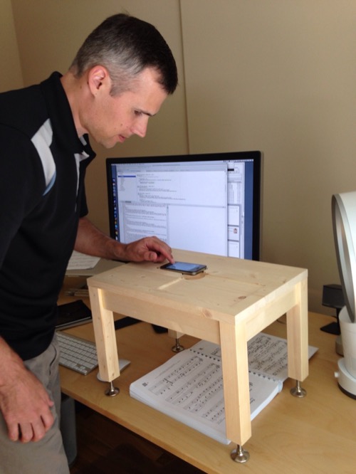
My custom built iTable™
The table has cutout insets on the top for an iPhone and an iPad mini, and a hole in centre for the camera.
Binarization Failures
I found two root causes of the binarization failures that I observed:
-
Background estimation by polynomial fitting is not robust when there are discontinuities in the background.
-
Otsu’s method is not robust when the image histogram is not bimodal.
In the following two sections I’ll elaborate on these problems.
The Problem with Background Estimating with Polynomials
The problem with estimating the background with a polynomial is the assumption of “smoothness” (or what mathematicians call continuity). In most cases when a page is placed in a well lit environment suitable for taking pictures, the background of a document image is smooth. Any variation that is observed usually comes from some curvature in the paper caused by the binding. But there are a few real-world scenarios that can cause the background to have a discontinuity:
-
A sharp shadow cast on the image.
-
The camera’s field of view extending beyond the bounds of the page, thus capturing either a portion of the opposing page in a book or the surface the book is on.
I’m going to focus on the latter case, as this is the problem that I encountered. Figure 10 shows an example of an image that includes a bit of the opposing left page. The binding caused the right side of the left page to be oriented perpendicular to the light source, making it significantly brighter than any other part of the image. Likewise, the left side of the right page received the least amount of light. Consequently, on the boundary between the left and right page there’s a sharp discontinuity, with the image’s lightest and darkest pixels on either side. Fitting a polynomial to this background will inevitably have a large error at points near the discontinuity. This is evident in Figure 11 which shows the result of Lu’s algorithm.
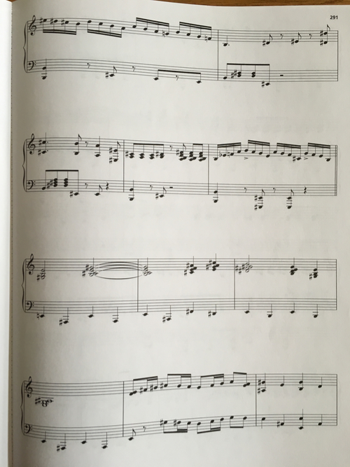
Image of a right-side page that also includes part of the opposing left-side page.
The book binding causes opposing pages to have significantly different illumination from the light source along the binding, causing a discontinuity in the image intensity.
Results of applying Lu’s algorithm on the image in Figure 10.
The Problem with Using Otsu’s Method Globally
As mentioned earlier, Otsu’s method assumes the image’s histogram is bimodal. I was able to tweak some aspects of the background polynomial fitting to minimize the effects of the discontinuity sufficiently to obtain what appeared to be a good normalized image. Figure 12 shows a normalized image.
Normalized image.
The histogram for this image is shown below. The histogram is trimodal (or arguably it has four modes). The most prominent mode—representing the background—is near 130; the foreground pixels form a barely visible and very broad distribution centred near 35; and there is a cluster of pixels at 255 which is from the bright strip along the left edge. By Otsu’s method the optimal threshold here is at 187, which is on the wrong side of the big hump and produces an almost entirely black binary image. A threshold near 80 is almost as good by Otsu’s statistical measure. It turns out that if the fitted background polynomial is varied just a bit, the normalized image will be a little bit different, and Otsu’s method will find a good threshold on the left side of the hump.

The graylevel histogram for image in Figure 12.
The issue is that Otsu’s method assumes a bimodal histogram, and we won’t always get that. If we assume our documents have a white background and that there are significantly more background pixels than foreground pixels then the most prominent mode in the image histogram will represent the background. The threshold we’re looking for must be smaller than the primary mode. So, we can just apply Otsu’s method to the subset of the image histogram in the interval \([0, b]\) where \(b\) is the location of the most prominent mode.
A New Approach
The new binarization technique that I now use with Music Lens is still based on polynomial fitting and Otsu’s method, but in a completely different way than employed by Lu. The algorithm was inspired by another paper by Lu et al. titled Document image binarization using background estimation and stroke edges [3]. (Of note, the algorithm described in this paper won the 2009 DIBCO.) Although my algorithm abandons the use of background estimation and image normalization, it adopts the idea of using edges. The general approach is to find a suitable thresholding function \(T\) that allows the binary image to be computed as:
The function \(T\) is obtained as follows:
-
Let \(S\) be the image produced by applying a Sobel filter to image \(I\). This finds pixels that are likely edge pixels (i.e. pixels at the boundary between the foreground and background). Otsu’s method is applied to \(S\), yielding \(S'\). The pixels in \(S'\) with the value 1 are likely edge pixels. (Any other standard edge detection algorithm should also suffice here.)
-
For each point \((x, y)\) where \(S'(x, y) = 1\), we apply Otsu’s method to a small (\(33 \times 33\)) window centred at \((x, y)\) in the original image \(I\). This gives us a set of points in \(\mathbb{R}^3\) \(U = \{(x_i, y_i, t_i)\}\) where \(t_i\) is the optimal threshold near \((x_i, y_i)\).
-
Let \(Q\) be the bivariate polynomial of degree 3 fitted to the points in \(U\).
-
Define \(T\) as:
\[ T(x, y) = \left\{ \begin{array}{ll} Q(x, y) & \text{if $D(x, y) < k$} \\ 0 & \text{if $D(x, y) \ge k$} \end{array} \right. \]where \(D(x, y)\) is the shortest distance between \((x, y)\) and any point in \(U\) (ignoring the \(z\) coordinate \(t_i\)). \(k\) is a parameter that effectively limits the domain of \(Q\) to points that are close to an edge. If we are far from an edge, the value of \(Q\) is unpredictable. We can conclude, however, that points far from an edge must be background points. This does assume that the document’s foreground is limited to thin stroke-based glyphs, which is a reasonable assumption for text documents. For music scores, setting \(k\) proportional to the staff line spacing is more appropriate, since the thickest “stroke” found in music notation is not larger than a staff space. How to pick \(k\) for both text and music scores will be explained below.
Let’s examine how this algorithm works for the image in Figure 11, which Lu’s algorithm did poorly on. First we apply edge detection to the original image; the result is shown in Figure 14.
Results of applying edge detection to the image in Figure 11.
Rather than compute the function \(D\) directly, we can construct a binary image that indicates whether \(D(x, y) \lt k\). If \(D(x, y) \lt k\), then the pixel value at \((x, y)\) is 1; otherwise the pixel value is 0. Such an image can easily be constructed by dilating the image \(S'\) with a box of width \(2k\); the result of this dilation is shown in Figure 15.
Results of dilating the edge image in Figure 14.
The white pixels define the domain where the function Q is valid.
But how is \(k\) chosen? The parameter \(k\) should be several times larger than the dominant stroke width. The technique in [3] estimates \(k\) by examining the horizontal or vertical distance between adjacent edge pixels. If we plot a histogram of these distances, the stroke width is estimated by the most frequent distance (the location of the highest peak in the histogram). For music scores, I use a variation of the same technique and use the second highest peak in the histogram, which corresponds to the staff line spacing. The histogram for the edge image in Figure 14 is shown below (Figure 16).

Histogram of vertical distances between adjacent edges.
The higest peak, at 2, corresponds to the dominant stroke thickness. In the case of music scores, this is the general line thickness (staff lines, bar lines, etc.); in a text document, it would be the stroke thickness of letters. The next peak, at 19, corresponds to the space between staff lines; this is the value of \(k\) we use for music scores.
The final binary image produced by using the thresholding function \(T\) is shown in Figure 17. Although there is still some noise along the binding, all of the music notation is clearly rendered.
The final binarized image using the new algorithm.
As I mentioned earlier, document binarization is currently an active research area. I’m more practitioneer than researcher, so I haven’t read all the recent literature on the topic. Of the many papers I have read though, those by Lu et al. have been the most influential on my own experimentation. Early on I selected their algorithm from [2] for Music Lens because it was conceptually elegant and fast. As I started to experiment with algorithms of my own design, I borrowed many ideas from Lu’s later work [3], notably using edge detection and employing a histogram of adjacent edge distances. My focus is now on finishing Music Lens rather than doing more exploration of binarization algorithms. But, I welcome any feedback from readers on the topic.
References
[1] Otsu, N. 1979. “A Threshold Selection Method From Gray-Level Histogram.” 9 (1). IEEE Transanctions on Systems, Man, and Cybernetics: 62–66.
[2] Lu, S., and C.L. Tan. “Thresholding of Badly Illuminated Document Images Through Photometric Correction.” Proceedings of the 2007 ACM Symposium on Document Engineering, 2007, 3–8.
[3] Lu, Shijian, Bolan Su, and Chew Lim Tan. “Document Image Binarization Using Background Estimation and Stroke Edges.” Ijdar 13, no. 4 (October 21, 2010): 303–14.